Analyzing Experiments Using the marginaleffects Package for R

By Vincent Arel-Bundock

Vincent Arel-Bundock will provide hands-on exercises and more insights for analyzing experiments using the marginaleffects package for R during the Interpreting and Communicating Statistical Results with R short course on June 18-21.

2×2 Experiments

A 2×2 factorial design is a type of experimental design that allows researchers to understand the effects of two independent variables (each with two levels) on a single dependent variable. The design is popular among academic researchers as well as in industry when running A/B tests.

In this blog, we illustrate how to analyze these designs with the the marginaleffects package for R. As we will see, marginaleffects includes many convenient functions for analyzing both experimental and observational data, and for plotting our results.

Fitting a Model

We will use the mtcars dataset. We’ll analyze fuel efficiency, mpg (miles per gallon), as a function of am (transmission type) and vs (engine shape).

vs is an indicator variable for if the car has a straight engine (1 = straight engine, 0 = V-shaped). am is an indicator variable for if the car has manual transmission (1 = manual transmission, 0=automatic transmission). There are then four types of cars (1 type for each of the four combinations of binary indicators).

Let’s start by creating a model for fuel efficiency. For simplicity, we’ll use linear regression and model the interaction between vs and am.

library(tidyverse) 
library(marginaleffects) 
library(modelsummary)  

## See ?mtcars for variable definitions 
fit <- lm(mpg ~ vs + am + vs:am, data=mtcars) # equivalent to ~ vs*am

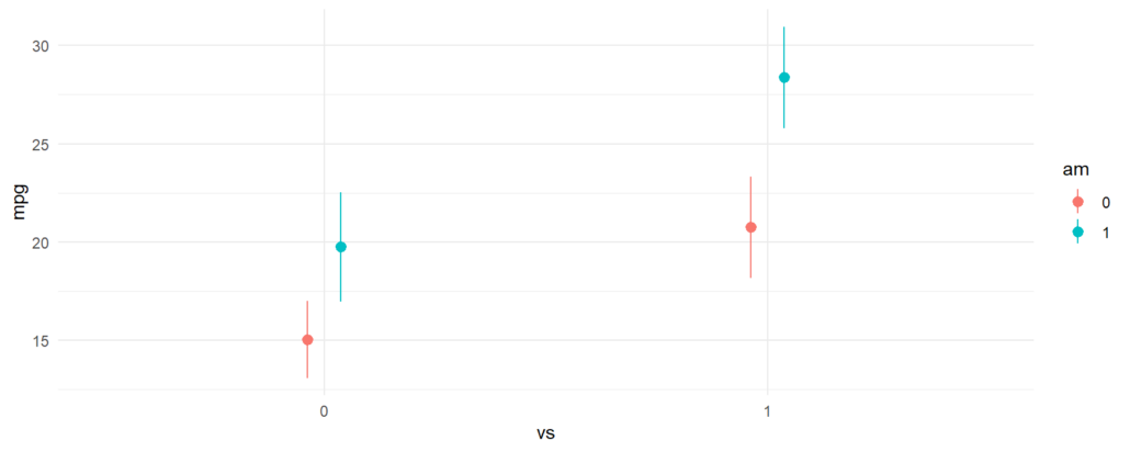
We can plot the predictions from the model using the plot_predictions function. From the plot below, we can see a few things:

Straight engines (vs=1) are estimated to have better expected fuel efficiency than V-shaped engines (vs=0).
Manual transmissions (am=1) are estimated to have better fuel efficiency for both V-shaped and straight engines.
For straight engines, the effect of manual transmissions on fuel efficiency seems to increase.

plot_predictions(fit, by = c("vs", "am"))

Evaluating Effects From The Model Summary

Since this model is fairly simple, the estimated differences between any of the four possible combinations of vs and am can be read from the regression table, which we create using the modelsummary package:

modelsummary(fit, gof_map = c("r.squared", "nobs"))

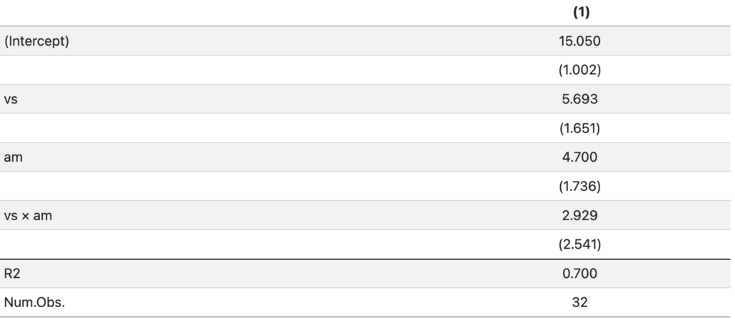
We can express the same results in the form of a linear equation:

With a little arithmetic, we can compute estimated differences in fuel efficiency between different groups:

4.700 mpg between am=1 and am=0, when vs=0.
5.693 mpg between vs=1 and vs=0, when am=0.
7.629 mpg between am=1 and am=0, when vs=1.
8.621 mpg between vs=1 and vs=0, when am=1.
13.322 mpg between a car with am=1 and vs=1, and a car with am=0 and vs=0.

Reading off these differences from the model summary is relatively straightforward in very simple cases like this one. However, it becomes more difficult as more variables are added to the model, not to mention obtaining estimated standard errors becomes nightmarish. To make the process easier, we can leverage the avg_comparisons() function from the marginaleffects package to compute the appropriate quantities and standard errors.

Using avg_comparisons To Estimate All Differences

The grey rectangle in the graph below is the estimated fuel efficiency when vs=0 and am=0, that is, for an automatic transmission car with a V-shaped engine.

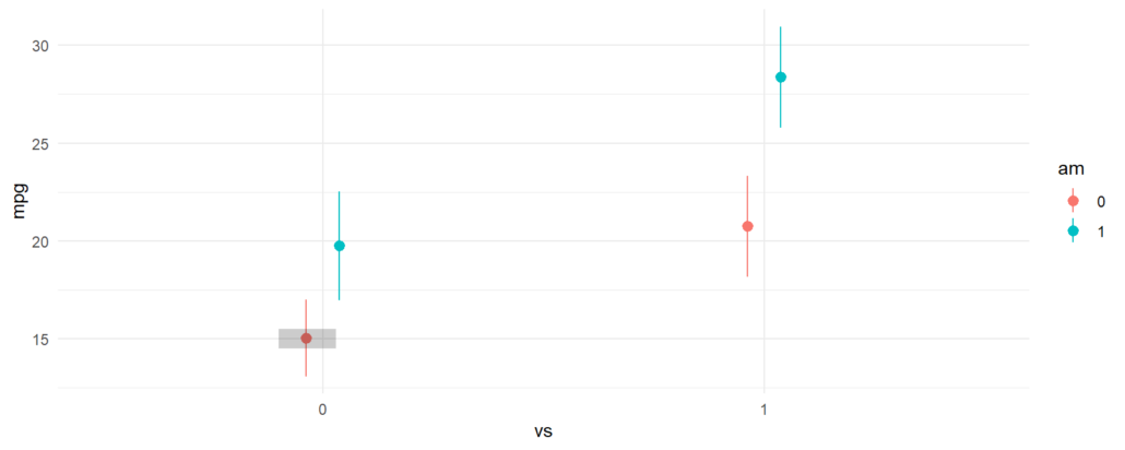
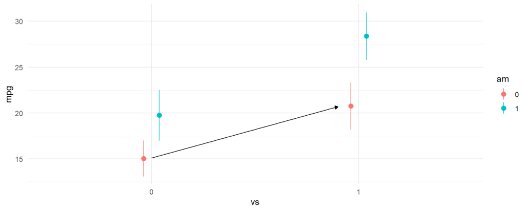
Let’s use avg_comparisons to get the difference between straight engines and V-shaped engines when the car has automatic transmission. In this call, the variables argument indicates that we want to estimate the effect of a change of 1 unit in the vs variable. The newdata=datagrid(am=0) determines the values of the covariates at which we want to evaluate the contrast.

avg_comparisons(fit,
variables = "vs",
newdata = datagrid(am = 0))
#> 
#> Term Contrast Estimate Std. Error z Pr(>|z|) S 2.5 % 97.5 %
#> vs 1 - 0 5.69 1.65 3.45 <0.001 10.8 2.46 8.93
#> 
#> Columns: rowid, term, contrast, estimate, std.error, statistic, p.value, s.value, conf.low, conf.high, predicted, predicted_hi, predicted_lo

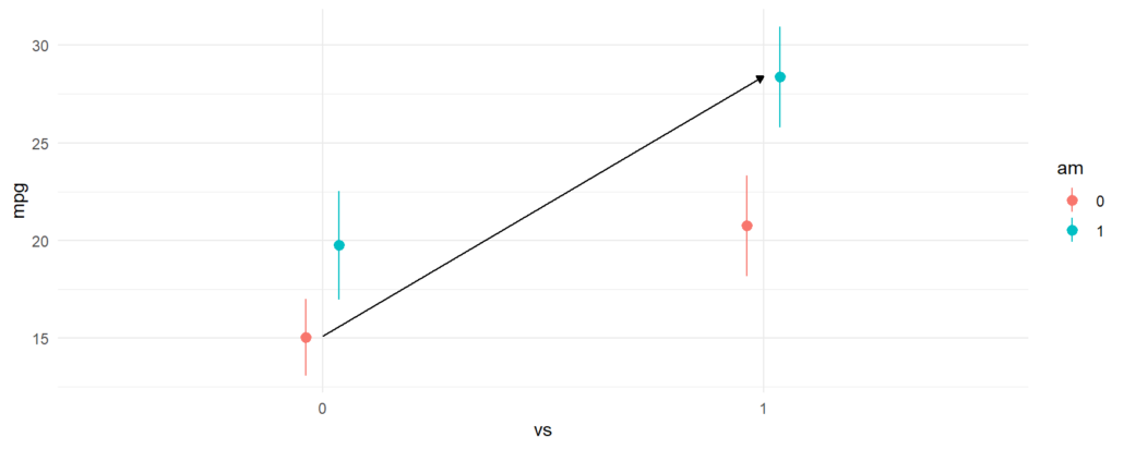
As expected, the results produced by avg_comparisons() are exactly the same as those which we read from the model summary table. The contrast that we just computed corresponds to the change illustrasted by the arrow in this plot:

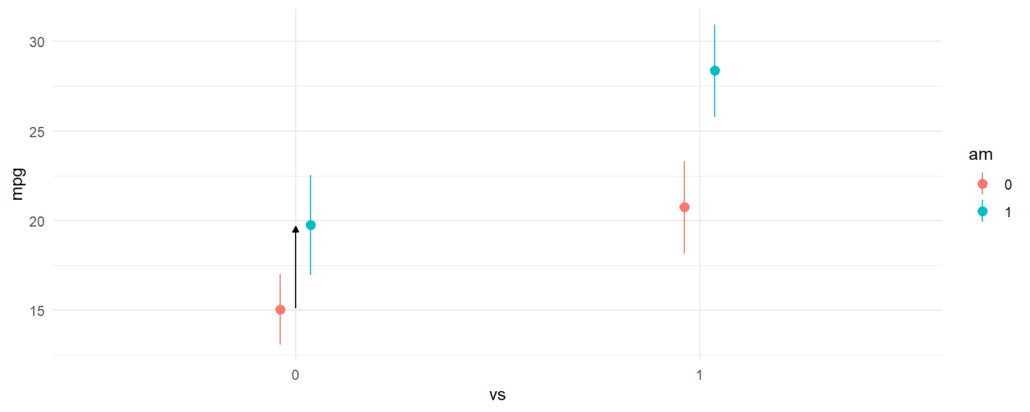
The next difference that we compute is between manual transmissions and automatic transmissions when the car has a V-shaped engine. Again, the call to avg_comparisons is shown below, and the corresponding contrast is indicated in the plot below using an arrow.

avg_comparisons(fit,
variables = "am",
newdata = datagrid(vs = 0))
#> 
#> Term Contrast Estimate Std. Error z Pr(>|z|) S 2.5 % 97.5 %
#> am 1 - 0 4.7 1.74 2.71 0.00678 7.2 1.3 8.1
#> 
#> Columns: rowid, term, contrast, estimate, std.error, statistic, p.value, s.value, conf.low, conf.high, predicted, predicted_hi, predicted_lo

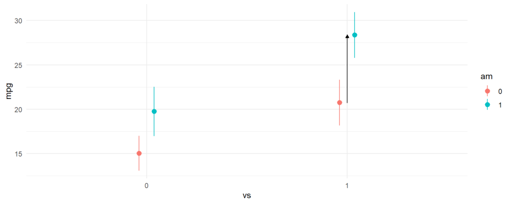
The third difference we estimated was between manual transmissions and automatic transmissions when the car has a straight engine. The model call and contrast are:

avg_comparisons(fit,
variables = "am",
newdata = datagrid(vs = 1))
#> 
#> Term Contrast Estimate Std. Error z Pr(>|z|) S 2.5 % 97.5 %
#> am 1 - 0 7.63 1.86 4.11 <0.001 14.6 3.99 11.3
#> 
#> Columns: rowid, term, contrast, estimate, std.error, statistic, p.value, s.value, conf.low, conf.high, predicted, predicted_hi, predicted_lo

The last difference and contrast between manual transmissions with straight engines and automatic transmissions with V-shaped engines. We call this a “cross-contrast” because we are measuring the difference between two groups that differ on two explanatory variables at the same time. To compute this contrast, we use the cross argument of avg_comparisons:

avg_comparisons(fit,
variables = c("am", "vs"),
cross = TRUE)
#> 
#> C: am C: vs Estimate Std. Error z Pr(>|z|) S 2.5 % 97.5 %
#> 1 - 0 1 - 0 13.3 1.65 8.07 <0.001 50.3 10.1 16.6
#> 
#> Columns: term, contrast_am, contrast_vs, estimate, std.error, statistic, p.value, s.value, conf.low, conf.high

Conclusion

The 2×2 design is a very popular design, and when using a linear model, the estimated differences between groups can be directly read off from the model summary, if not with a little arithmetic. However, when using models with a non-identity link function, or when seeking to obtain the standard errors for estimated differences, things become considerably more difficult. This vignette showed how to use avg_comparisons to specify contrasts of interests and obtain standard errors for those differences. The approach used applies to all generalized linear models and effects can be further stratified using the by argument (although this is not shown in this vignette.)